Tutorial
Basic usage with an example dataset. Note, this tutorial uses the
matplotlib graphing module which is not a dependency of AeroEvap,
be sure to install it to your environment before running this tutorial
if you want the plots to display correctly.
>>> import pandas as pd
>>> import numpy as np
>>> from aeroevap import Aero
>>> from IPython.display import IFrame
>>> import matplotlib.pyplot as plt
>>> %matplotlib inline
Example data
This example uses buoy data from a location near Savannah, GA (NOAA station ID is 41008). The buoy is maintained by the National Data Buoy Center (NDBC), more buoy information is shown in the embedded page below. The meterological data used in this example is hosted by NOAA and downloaded directly and formatted for a month of data.
The line below downloads the time series of current year buoy standard meterological data directly from the NDBC.
Input units:
WDIR |
WSPD |
GST |
WVHT |
DPD |
APD |
MWD |
PRES |
ATMP |
WTMP |
DEWP |
VIS |
TIDE |
|---|---|---|---|---|---|---|---|---|---|---|---|---|
degT |
m/s |
m/s |
m |
sec |
sec |
deg |
hPa |
degC |
degC |
degC |
nmi |
ft |
>>> # get standard meterological data from National Data Buoy Center
>>> met_df = pd.read_csv(
>>>     'https://www.ndbc.noaa.gov/data/l_stdmet/41008.txt',
>>>     delim_whitespace=True, skiprows=[1], na_values=[999.0]
>>> )
Make a datetime index and clean up the dataframe.
>>> met_df.index = pd.to_datetime(
>>>     dict(
>>>         year=met_df['#YY'],
>>>         month=met_df.MM,
>>>         day=met_df.DD,
>>>         hour=met_df.hh,
>>>         minute=met_df.mm
>>>     )
>>> )
>>> met_df.index.name = 'date'
>>> met_df.drop(['#YY','MM','DD','hh','mm'], axis=1, inplace=True)
>>> met_df.head()
| WDIR | WSPD | GST | WVHT | DPD | APD | MWD | PRES | ATMP | WTMP | DEWP | VIS | TIDE | |
|---|---|---|---|---|---|---|---|---|---|---|---|---|---|
| date | |||||||||||||
| 2021-01-31 23:50:00 | 207 | 7.0 | 8.3 | 1.52 | 5.88 | 4.90 | 162 | 1009.1 | 15.9 | 13.6 | 14.3 | 99.0 | 99.0 |
| 2021-02-01 00:50:00 | 208 | 8.0 | 9.9 | 1.38 | 6.67 | 4.91 | 143 | 1008.6 | 15.7 | 13.6 | 14.3 | 99.0 | 99.0 |
| 2021-02-01 01:50:00 | 216 | 10.3 | 11.8 | 1.58 | 6.25 | 4.79 | 157 | 1007.8 | 17.2 | 13.7 | 15.7 | 99.0 | 99.0 |
| 2021-02-01 02:50:00 | 273 | 8.5 | 11.6 | 1.55 | 5.88 | 5.01 | 151 | 1008.3 | 15.9 | 13.7 | 15.0 | 99.0 | 99.0 |
| 2021-02-01 03:50:00 | 320 | 2.5 | 3.5 | 1.45 | 6.67 | 5.43 | 140 | 1008.5 | 14.6 | 13.7 | 14.6 | 99.0 | 99.0 |
Because the input dataset does not include relative humitidy we can estimate it using an approximation to the Clausius–Clapeyron relation using air and dewpoint temperatures. Relative humitidy is needed in the aerodynamic mass-transfer evaporation calculations.
>>> # vapor pressure and saturation vapor pressure using Clausius–Clapeyron relation
>>> met_df['e'] = 0.611 * np.exp( 5423 * ((1/273) - (1/(met_df.DEWP+273.15))) )
>>> met_df['es'] = 0.611 * np.exp( 5423 * ((1/273) - (1/(met_df.ATMP+273.15))) )
>>> # calculate relative humitidy
>>> met_df['RH'] = 100 * (met_df.e/met_df.es)
>>> plt.figure(figsize=(8,4))
>>> met_df.RH.plot()
>>> plt.ylabel('estimated relative humitidy')
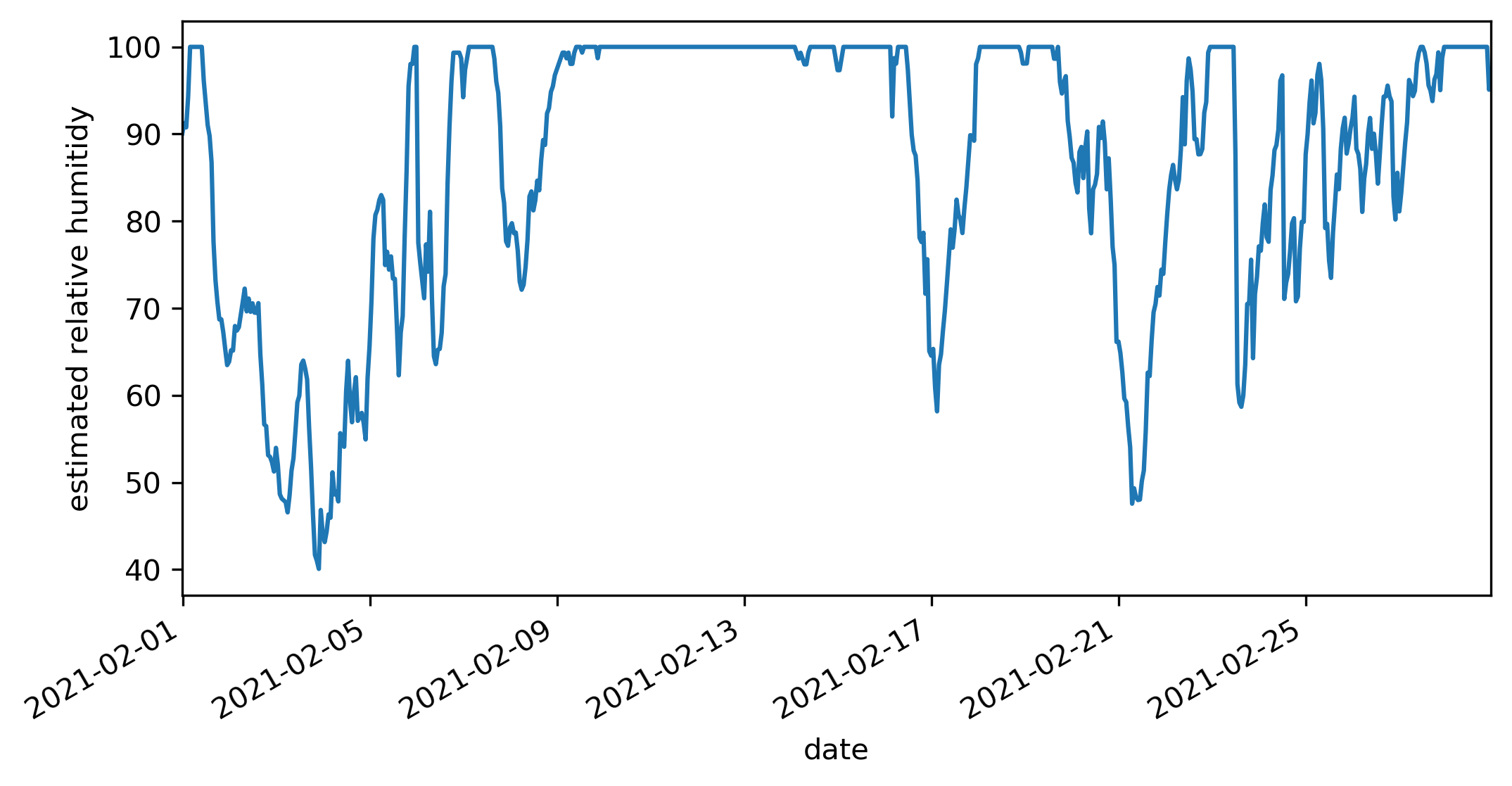
In this case we do not need to convert air pressure to millibars because 1 hPa = 1 mbar.
Create an Aero object
The Aero object allows for loading a pandas.DataFrame containing
meterological data required for calculating aerodynamic mass-transfer
open water evaporation in parrallel. The object can be initialized from
a pandas.DataFrame or the pandas.DataFrame can be assigned
later, e.g.
>>> Aero_empty = Aero()
>>> Aero_with_df = Aero(met_df)
>>> Aero_empty.df is None
    True
>>> # the df property can be assigned after initialization:
>>> Aero_empty.df = met_df
>>> # the data has been added
>>> Aero_empty.df.head()
| WDIR | WSPD | GST | WVHT | DPD | APD | MWD | PRES | ATMP | WTMP | DEWP | VIS | TIDE | e | es | RH | |
|---|---|---|---|---|---|---|---|---|---|---|---|---|---|---|---|---|
| date | ||||||||||||||||
| 2021-01-31 23:50:00 | 207 | 7.0 | 8.3 | 1.52 | 5.88 | 4.90 | 162 | 1009.1 | 15.9 | 13.6 | 14.3 | 99.0 | 99.0 | 1.658512 | 1.841077 | 90.083807 |
| 2021-02-01 00:50:00 | 208 | 8.0 | 9.9 | 1.38 | 6.67 | 4.91 | 143 | 1008.6 | 15.7 | 13.6 | 14.3 | 99.0 | 99.0 | 1.658512 | 1.817315 | 91.261670 |
| 2021-02-01 01:50:00 | 216 | 10.3 | 11.8 | 1.58 | 6.25 | 4.79 | 157 | 1007.8 | 17.2 | 13.7 | 15.7 | 99.0 | 99.0 | 1.817315 | 2.002412 | 90.756312 |
| 2021-02-01 02:50:00 | 273 | 8.5 | 11.6 | 1.55 | 5.88 | 5.01 | 151 | 1008.3 | 15.9 | 13.7 | 15.0 | 99.0 | 99.0 | 1.736292 | 1.841077 | 94.308483 |
| 2021-02-01 03:50:00 | 320 | 2.5 | 3.5 | 1.45 | 6.67 | 5.43 | 140 | 1008.5 | 14.6 | 13.7 | 14.6 | 99.0 | 99.0 | 1.691456 | 1.691456 | 100.000000 |
You may only assign a pandas.DataFrame to Aero.df,
>>> # this will not work, df needs to be a dataframe
>>> Aero_empty.df = 'high five'
---------------------------------------------------------------------------

TypeError                                 Traceback (most recent call last)

<ipython-input-13-5de371e56275> in <module>
      1 # this will not work, df needs to be a dataframe
----> 2 Aero_empty.df = 'high five'


~/AeroEvap/aeroevap/aero.py in df(self, df)
    122     def df(self, df):
    123         if not isinstance(df, pd.DataFrame):
--> 124             raise TypeError("Must assign a pandas.DataFrame object")
    125         self._df = df
    126


TypeError: Must assign a pandas.DataFrame object
Input variables and units
The meterological variables needed for running the aerodynamic mass-transfer estimation of evaporation are the following:
variable |
units |
naming |
|---|---|---|
wind speed |
m/s |
WS |
air pressure |
mbar |
P |
air temperature |
C |
T_air |
skin temperature |
C |
T_skin |
relative humidity |
0-100 |
RH |
where the “naming” column refers to the internal names expected by the
Aero.run method, i.e. the column headers in the dataframe should
either be named accordingly or a dictionary that maps your column names
to those internal names can be passed (see examples below).
To run the evaporation calculation you will also need the anemometer height in meters and the temporal sampling frequency of the data in seconds.
Run calculation on time series
As mentioned, this dataset has unique naming conventions, therefore we need to tell AeroEvap which variables are which with a dictionary,
>>> # make a naming dict to match up columns with Aero variable names
>>> names = {
>>>     'WSPD' : 'WS',
>>>     'ATMP' : 'T_air',
>>>     'WTMP' : 'T_skin',
>>>     'PRES' : 'P'
>>> }
Alternatively you could rename wind speed, air and surface temperature, and air pressure columns to the apprpriate names specified in the table above in Input variables and units.
Now we are ready to run the aerodynamic mass-transer evaporation on the full time series in our dataframe. Lastly, the sensor height of the anemometer and temporal sampling frequency of the data needs to be supplied, in this case the height is 4 meters and the data frequency is 10 minutes or 600 seconds.
This example assumes there are 8 physical or logical processors
available for parallelization, if not specified the Aero.run routine
will attempt to use half of the available processors.
>>> np.seterr('ignore')
>>> # create a new Aero object and calculate evaporation on all rows
>>> A = Aero(met_df)
>>> A.run(sensor_height=4, timestep=600, variable_names=names)
After the calculations are complete three variables will be added to the Aero.df dataframe: ‘E’, ‘Ce’, ‘VPD’, and ‘stability’ which are evaporation in mm/timestep, bulk transfer coefficient, vapor pressure deficit (kPa), and the Monin-Obhukov Similarity Theory (MOST) stability parameter (z/L).
>>> A.df[['E', 'Ce', 'VPD', 'stability']].head()
| E | Ce | VPD | stability | |
|---|---|---|---|---|
| date | ||||
| 2021-01-31 23:50:00 | -0.002865 | 0.001296 | -0.069970 | 0.075544 |
| 2021-02-01 00:50:00 | -0.003473 | 0.001368 | -0.070289 | 0.048386 |
| 2021-02-01 01:50:00 | -0.014245 | 0.001443 | -0.213278 | 0.042489 |
| 2021-02-01 02:50:00 | -0.007264 | 0.001391 | -0.136129 | 0.043363 |
| 2021-02-01 03:50:00 | -0.000994 | 0.000932 | -0.094175 | 0.367295 |
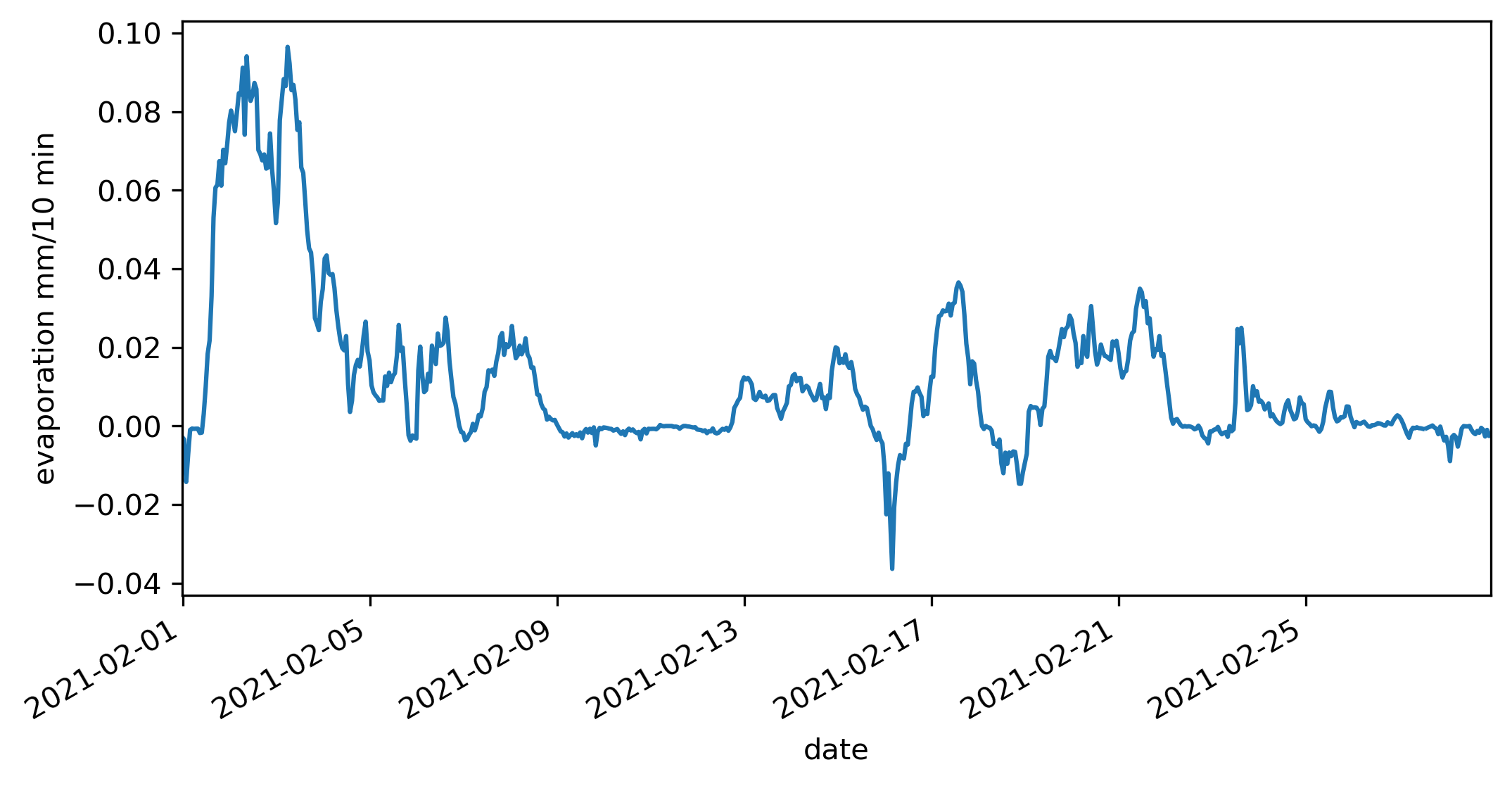
View the calculated evaporation,
>>> plt.figure(figsize=(8,4))
>>> A.df.E.plot()
>>> plt.ylabel('evaporation mm/10 min')
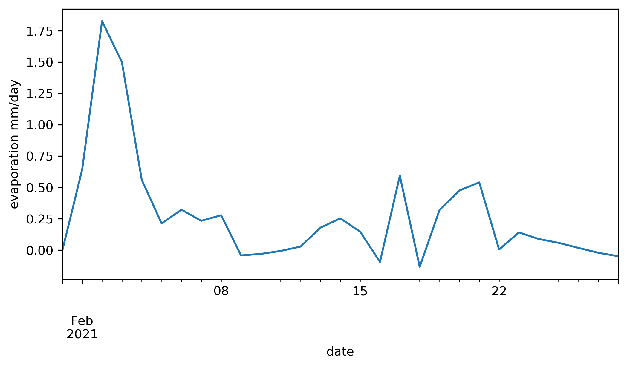
The calculated open-water evaporation is shown below after creating a daily sum.
>>> plt.figure(figsize=(8,4))
>>> A.df.E.resample('D').sum().plot()
>>> plt.ylabel('evaporation mm/day')
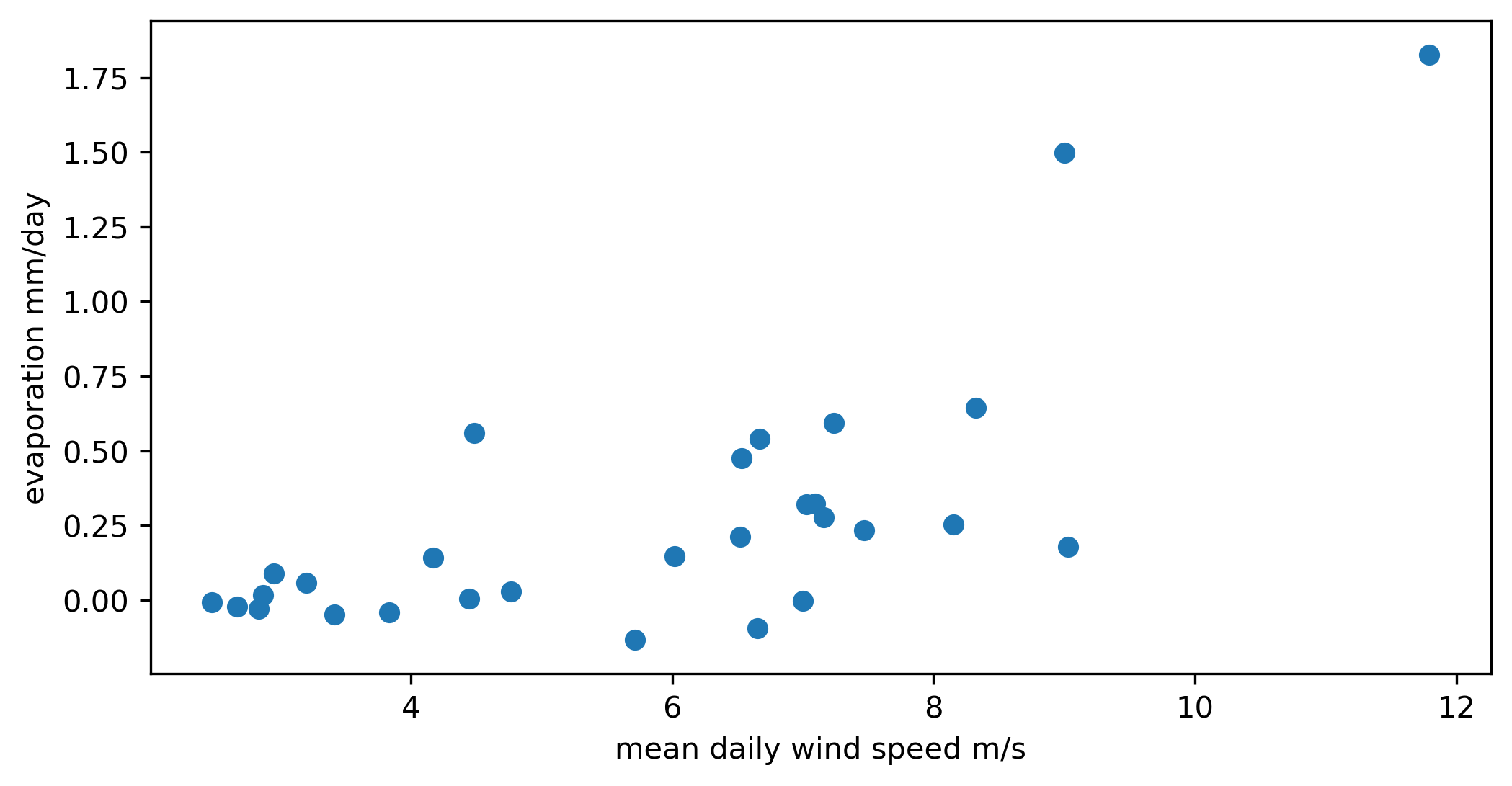
And the wind speed relation versus the calculated evaporation.
>>> plt.figure(figsize=(8,4))
>>> plt.scatter(A.df.WSPD.resample('D').mean(), A.df.E.resample('D').sum())
>>> plt.ylabel('evaporation mm/day')
>>> plt.xlabel('mean daily wind speed m/s')
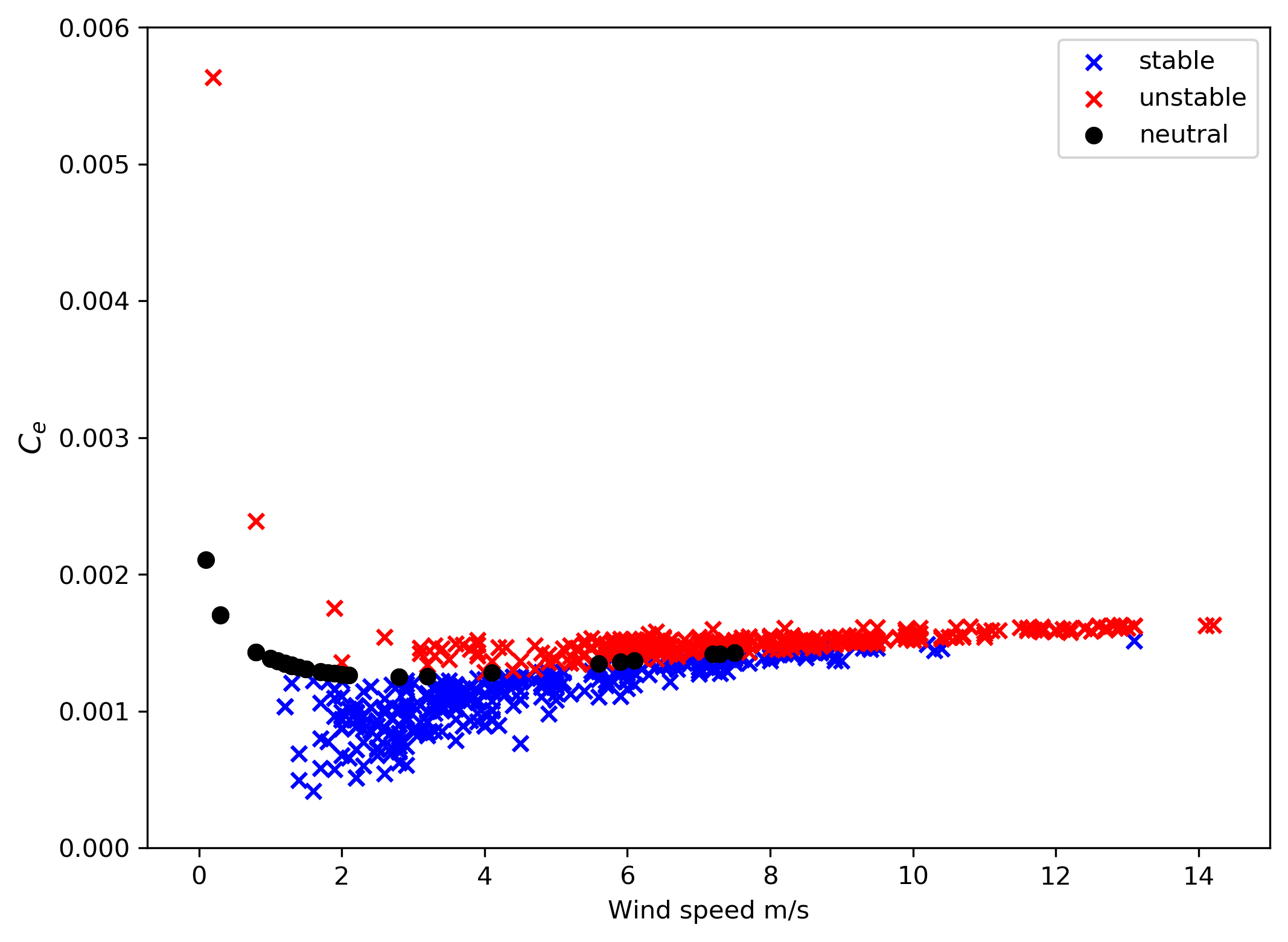
We can use the MOST stability parameter for relating the wind speed to the bulk transfer coefficient as well by classifying them by unstable, stable, and neutral conditions.
>>> stable = np.real(A.df.stability) > 0
>>> unstable = np.real(A.df.stability) < 0
>>> neutral = np.real(A.df.stability) == 0
>>> plt.figure(figsize=(8,6))
>>> plt.scatter(A.df.WSPD[stable], A.df.Ce[stable], marker='x', color='blue', label='stable')
>>> plt.scatter(A.df.WSPD[unstable], A.df.Ce[unstable], marker='x', color='red', label='unstable')
>>> plt.scatter(A.df.WSPD[neutral], A.df.Ce[neutral], marker='o', color='black', label='neutral')
>>> plt.ylim(0,0.006)
>>> plt.ylabel(r'$C_e$', fontsize=12)
>>> plt.xlabel('Wind speed m/s')
>>> plt.legend()
Single calculation
The Aero class also provides a method Aero.single_calc that can
be used on a single set of meterological data to calculate the
instantaneous open-water evaporation. It requires the same inputs as
Aero.run however the inputs are scalars as opposed to time series.
For example using the first timestamp of our example buoy data we can
calculate E, Ce, VPD, and stability:
>>> datetime = '2019-08-01 00:00:00'
>>> wind = 3.3
>>> pressure = 1021.2
>>> T_air = 18.1
>>> T_skin = 18.4
>>> RH = 80.26
>>> sensor_height = 4
>>> timestep = 600
>>> E, Ce, VPD, stability = Aero.single_calc(
>>>     datetime,
>>>     wind,
>>>     pressure,
>>>     T_air,
>>>     T_skin,
>>>     RH,
>>>     sensor_height,
>>>     timestep
>>> )
>>> E, Ce, VPD, stability
    (0.008724959939647368, 0.001310850807452679, 0.44947250457458576, -0.049355020952319244)
Theory behind calculations
This is a work in progress, for now please refer to references hosted on GitHub about the methodologies used.